QDpack example - Coupled qubits

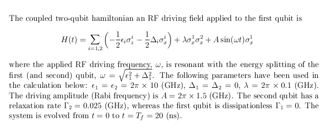
This document describes how to use the QD package to calculate the dynamics of a simple quantum system. The example is a system of two coupled qubits that are initially in their ground states. An RF field is applied to the first qubit which gradually excite it (Rabi oscillations). The static interaction between the qubits cause energy exchange between the qubit once energy is pumped into the first qubit via the RF field. The example program is configured to output the occupation probabilities for each qubit.

Model and parameter values

The model and parameter values used in this example are the following:

Example source code

The example programs source code is available for download here, and it is also available in the QDpack source code distribution.

Program structure

First the parameters for the Hamiltonian is configured by initializing a data structure of the type "solver_param".
Next, a Hamiltonian is set up (either a new Hamiltonian is implemented, or one from the QDpack library is used).
The quantum system data structure is created and initialized, i.e., the number of quantum levels in each subsystem is configured.
Dissipation is configured: A list of operators and rates that appear in the master equation (OPTIONAL).
Initial state is configured.
Finally, the solver is called. For each time-step the solver call a callback function where application specific processing of the density matrix at time t (extraction of occupation probabilites, calculation of expectation values, etc.) is be done.

Build and run

Build the example by typing "make run_qubits" in the QDpack directory. This will produce a executable file called "run_qubits". Run this program from the same directory, after making sure that the data output directory (data/qubit.dynamics) exists:

$ mkdir -p data/qubit.dynamics
$ time ./run_qubits
Quantum system with 2 sub systems: 2 2
DEBUG: combining (tensor product)
DEBUG: combining (tensor product)
DEBUG: starting dm_evolve_lme_t (Lindblad-type Master Eqaution)

real    0m1.078s
user    0m0.972s
sys     0m0.108s
$

The program output is stored in the directory data/qubit.dynamics/:

$ wc data/qubit.dynamics/*
1001  3003 27028 data/qubit.dynamics/qubit_population_0.dat
1001  3003 27028 data/qubit.dynamics/qubit_population_1.dat
3003  9009 81084 total
$

The occupation probabilities of each qubit is stored in individual files with and integer identifier in the file name. The data is formatted in the tab-separated values (TSV) ascii format, and column one to three is: 1) time, 2) probability to be in the ground state, and 3) probability of being in the excited state, respectively"

$ tail data/qubit.dynamics/qubit_population_0.dat
9.910000        0.869513        0.130487
9.920000        0.869527        0.130473
9.930000        0.869539        0.130461
9.940000        0.869553        0.130447
9.950000        0.869568        0.130432
9.960000        0.869587        0.130413
9.970000        0.869608        0.130392
9.980000        0.869634        0.130366
9.990000        0.869666        0.130334
10.000000       0.869703        0.130297
$

Plotting results

Plotting the results for the occupation probabilities for the three qubis gives the following figures:

$ enplot -x 0 -y 1,2 -X "time t (ns)" -Y "Occupation probabilities" -t "Occupation probability of qubit 1" -p qubit_1_populations.png data/qubit.dynamics/qubit_population_0.dat &
$ enplot -x 0 -y 1,2 -X "time t (ns)" -Y "Occupation probabilities" -t "Occupation probability of qubit 2" -p qubit_2_populations.png data/qubit.dynamics/qubit_population_1.dat &

Qubit 1 - populations as a function of time.

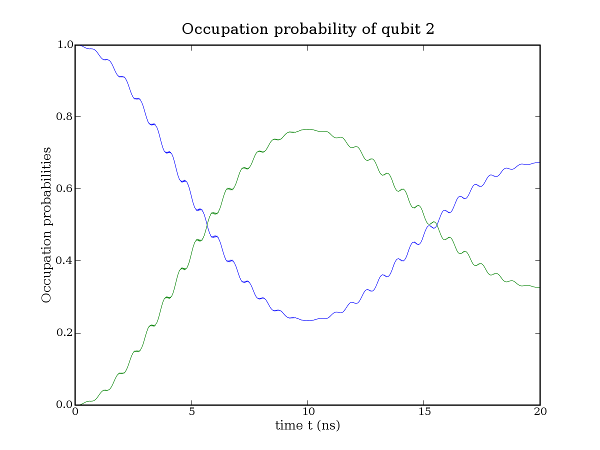
Figure caption: Left (top), the occupation probabilities of the first qubit. Fast oscillations are Rabi oscillations due to the RF driving. Slow oscillations are due to the static interaction with the second qubit. Right (bottom), the occupation probabilities of the second qubit. The oscillations are due to interaction with the first qubit. The gradual decay of oscillation visibility is due to dissipation in the second qubit (first qubit is dissipationless in this simulation).